Graphs For Beginners - Part-3

Types Of Graphs

We generally encounter the following types of graph in a problem. Each of them has some special properties which are often useful.

• Trees - This is by FAR the most common thing we shall encounter. Some don't even consider problems based on it as graph problems, still I will add this here for sake of completeness.
• Directed Acyclic Graphs (DAGs) - This is also a commonly recurring type of graph with lots of nice properties. For example, since cycles (acyclic .. duhh) do not exist, we are able to easily calculate DP on it. Later, we will show how ALL DP problems are just DAGs. 
• Planar graphs - These are quite rare but do appear in problems nonetheless. Special properties includes the application of euler's theorem and consideration of its dual graph.
• The vanilla version - This is our plain old graph, either directed or undirected. There are no special properties for this graph.
• Implicit graphs - sometimes the problem statement may not directly look like for a graph problem, but it often is.

Note that in each of these versions, the edges (or nodes) may have weights associated.

Don't worry, if something is not understood, I will probably go through these later. Or you can just google these yourself XD.

We will look at each of these separately.

Connected Components

Okay. So we have a graph. But what good does it do? Why is it even useful. Well... it can be used to answer many fundamental questions such as what is the shortest distance between two nodes, or whehter two nodes are even connected or not. 

Wait. What does it mean for two nodes to be connected? Let's introduce some new ideas:

• Path - We say that a path exist between two nodes u and v if we can go from u to v using one or more edges. For example, suppose we go form u-->a-->b-->v. Thus a path exists which connects u to v. Thus we say that v is "reachable" form u. Note that, in case of an undirected graph, this property is transitive: if u is reachable from v, then v is reachable from u. However that is not the case with directed graphs.
• Cycle - Now it may so happen that there exists such a path such that we can go from u to some vertex v and then again return to u without visiting any vertex twice. This is what we call a cycle. 
  
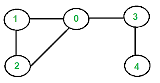  Here the nodes {0-->1 --> 2 --> 0} forms a cycle.
  
  
  
  

Connected components are a term that we use ONLY for Undirected graphs. (We will explore its counterpart in directed graphs later). It means a maximal set of nodes so that if we choose any two pair of nodes from them, we can go from one to the other.

Notice that suppose if we have a connected component C and a node u which has an edge to a node which is a part of C, then u can also be made a part of C. Herein the word maximal is important. It means that we extend our connected component as much as possible using the above method till no more nodes can be added in our connected component.

This graph, for example has 3 connected components.

So the question is, how to determine these connected components. 

Graph traversal

Graph traversal to the rescue. This is how we can ACTUALLY traverse the graph, kind of like a tourist who is visiting cities one by one. 

There are two types of graph traversals. Depth first search. And. Breadth first search. Let's look at each one by one.

DFS or Depth First Search

Here we start visiting the nodes one by one, unless we can no longer visit a previously unvisited node. 

The algorithm is basically like this:

Thus, suppose we start a DFS at node 1. Then we visit the first neighbour of node 1. Then we go to that Node, and again check all its neighbours. Note that we will not consider node 1 as its neighbour again because node 1 has already been marked as visited. Thus we will go to some other node, and from there to some other node.. and so on. However we will never enter a new recursion with a node that has already been visited.  This also guarentees that all nodes that are in the same connected component with the original node will get visited. that too, exactly once.  (Excercise?!)

Thus complexity of such a DFS is O(V + E) as we overall visit each node exactly once.. and in each node, although we go over all the edge, the sum of these edges is bounded by E. So we visit each node once and each edge atmost twice. (although we go through the edge exactly once.). Hence the complexity.

BFS or Breadth First search

Here, instead of trying to reach as many nodes as possible one by one, we go level by level. That is, we first visit the neighnour of our initial node. We call these nodes as being on depth 1. Now, we visit all the neighbours of these "depth-1" nodes. These will naturally be on depth 2. And so on and so forth. A question that can arise is.. suppose we visit a node at depth 6. Can't it be possible that it could also be visited at depth 4, or say depth 7? Well, here again we only visit unvisited nodes. So multiple depth assignments are not possible. Hence if it were possible to be visited in depth 4, we would actually have had visited it(think why). If it has been visited in depth 6, it would be pointless to again visit it at depth 7. This is because we generally want the shortest path to it.

I will just give a link to a nice tutorial about the actual algorithm to save some redundancy here.

Also, note that by doing a breadth first search from a node N, we actually get the shortest path to all nodes from it(the "depth number") in the connected component. This was however not the case with depth first search. Again, i'll leave this as an excercise as to why DFS is not sufficient. Oh, and note that BFS also marks the entire connected component. But it is seldom used as DFS is much shorter to code than BFS.